Swarm Robotics: First Exploration
Date:
Introduction
This project is led by a senior colleague in our laboratory. My primary contributions include wheeled robot control, EKF (Extended Kalman Filter) for position and heading smoothing, and potential field path planning. Check out our code here
Motion control for mobile robots
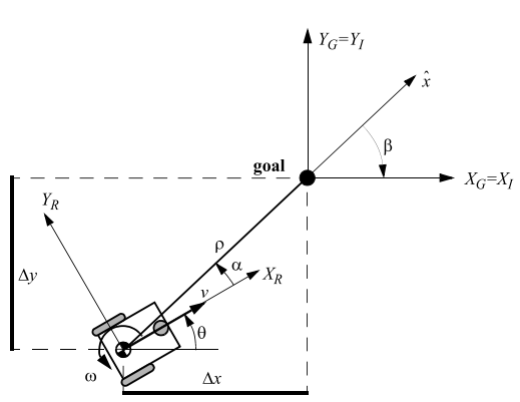
 \(r = 0.205\) m, \(l = 0.26\) m
In the context of linear control systems, where the outputs are velocity \(v\) and angular velocity \(\omega\), these need to be eventually converted into the rotational speeds of two wheels \(\varphi_1\) and \(\varphi_2\).
\(\displaylines{ \dot{\varphi_1} = \frac{1}{r}(v + l\omega)\\ \dot{\varphi_2} = \frac{1}{r}(v - l\omega) }\)
EKF Filter
When deploying a global camera to estimate the position and heading direction of the Epuck-2, we occasionally find that the estimation derived from the QR code introduces significant errors, potentially causing divergence and misalignment in fixed-point motion control. To improve motion stability and prevent such problems, we introduce an Extended Kalman Filter (EKF) to smooth the data.
Path Planning
Potential field path planning is a widely used algorithm that models a robot as a particle within a constructed potential field. This field is based on the distances between the robot’s current position, the target position, and any obstacles. The gradient of the potential field guides the robot’s movement towards the target. The steps for potential field path planning are as follows:
1. Construct the Potential Field:
Attractor (target): \(U_g(x, y) = \frac{1}{2}\kappa_g[(x - x_g)^2 + (y - y_g)^2]\)
Repeller (obstacles): \(U_o(x, y) = \left\{ \begin{array}{cl} \frac{1}{2}\kappa_o\left(\frac{1}{d} - \frac{1}{d_o}\right)^2 & \text{if }d < d_o \\ 0 & \text{otherwise} \end{array} \right.\)
Total Potential: \(U(x, y) = U_g(x, y) + \sum_{i=1}^n U_o(x, y)\)
2. Compute the Gradient: \(\nabla U(x, y) = \begin{pmatrix} \frac{\partial U}{\partial x} \\ \frac{\partial U}{\partial y} \end{pmatrix}\)
3. Path Calculation: \(\begin{bmatrix} \Delta x \\ \Delta y \end{bmatrix} = -\nabla U(x, y)\)
4. Robot Displacement Calculation: \(s = \sqrt{\Delta x^2 + \Delta y^2}, \quad \theta = \arctan\frac{\Delta x}{\Delta y}\)