
H-infinity Robust Controller Design
Date:
Design Procedure
Check out my MATLAB code on GitHub
Model linearization
Linearize a nonliear model on different equilibriums point(for unforced system, and \(\dot{x} = 0\)) and make a family of controller for each point. When operating our system, we need to switch between these linear models in order to have the best linear control for current operating point.
First-order Taylor series approximation(applying first-order Taylor approximation to 12 equations of motion (EOM)).
\[\displaylines{ \begin{bmatrix} M & 0_{6\times6}\\ 0_{6\times6} & I_{6\times6} \end{bmatrix} \begin{bmatrix} \dot{\nu}\\ \dot{\eta} \end{bmatrix} = \begin{bmatrix} (C+D)\nu - g(\eta) + \tau\\ J(\eta)\nu \end{bmatrix} }\] \[\displaylines{ Ef(\nu, \eta, t) = \begin{bmatrix} f_1(\nu, \eta, t)\\ f_2(\nu, \eta, t)\\ .\\ .\\ .\\ f_{12}(\nu, \eta, t) \end{bmatrix} }\] \[\displaylines{ \begin{split} \dot{x} &= E^{-1}Jacobian(f(\nu, \eta, t), \ x)x + E^{-1}Jacobian(f(\nu, \eta, t), \ u)u \\ y &= Cx \\ \end{split} }\] \[\displaylines{ \begin{split} A &= E^{-1}Jacobian(f(\nu, \eta, t), \ x)\\ B &= E^{-1}Jacobian(f(\nu, \eta, t),\ u) \end{split} }\]Here is an example :
% linearize by parameter matrix
% C(t)
fc = Cnu*nu
Ct = jacobian(fc,nu)

% D(t)
fd = Dnu*nu
Dt = jacobian(fd,nu)

% J(t)
fJ = J*nu
f_nu = jacobian(fJ, nu)
f_eta = jacobian(fJ, eta)

% linearized state-space representation of the full-order nonlinear model
Gss.A = double([-inv(M)*(C+D)  -inv(M)*G_t
                    Jnu           Jeta   ])
Gss.B = [inv(M);zeros(6)]
Gss.C = eye(12)
Gss.D = zeros(12,6)

Gss = ss(Gss.A,Gss.B,Gss.C,Gss.D)
H-infinity Loop Shaping Design (combining of mixsyn(performance) and ncfsyn(robustness))
uncertainty: co-prime factor uncertainty
control configuration: \(P-K\) structure
shaped plant: \(P_s = W_2 P W_1\) \(\quad P = \tilde{M}^{-1}\tilde{N}\)
final controller: \(K = W_1K_\infty W_2\)
property: obtain performance and robust stability trade-offs; loop shaping means shaping the magnitude of open loop transfer function \(L=GK\) as a function of frequency
Function:
ncfsyn(robustness)
loopsyn(performance and robustness)
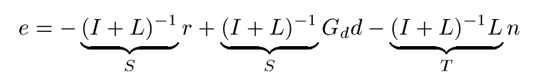
loop shaping method is based on analyzing open loop transfer function \(L\), however, at the crossover range where the magnitude of \(L\) is close to \(1\) one cannot infer anything about \(S\) and \(T\) from the magnitude of the loop shape \(\left| L(jw) \right|\), as a result, the crossover range maybe large which leads to a bad performance(large \(\gamma\) ). So an alternative design strategy is to directly shape the magnitudes of closed loop transfer functions, such as \(S(s)\) and \(T(s)\). And we can also combine mixed sensitivity and loop shaping.
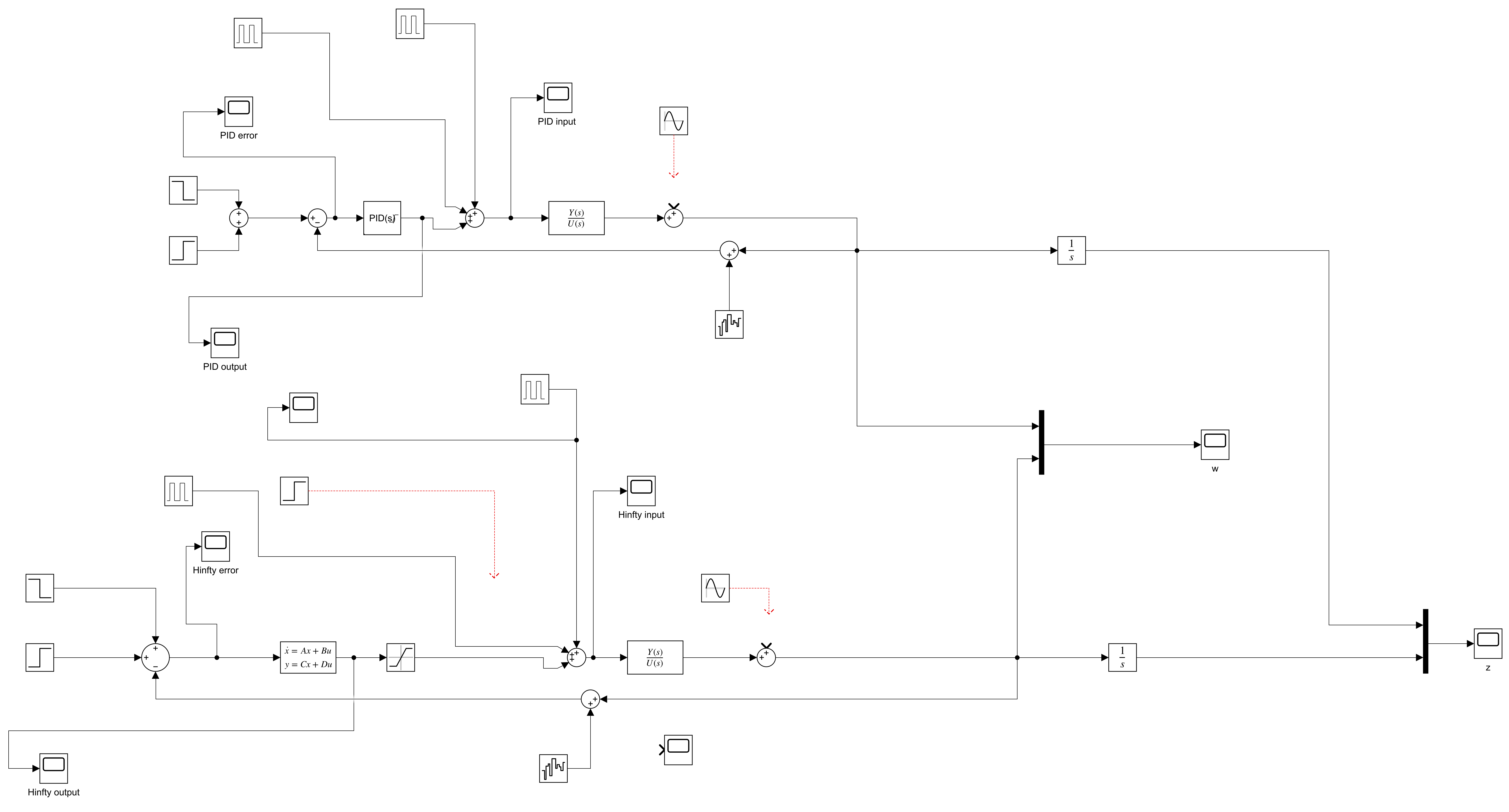
Implementation
Block diagrams in Simulink are shown as follows:
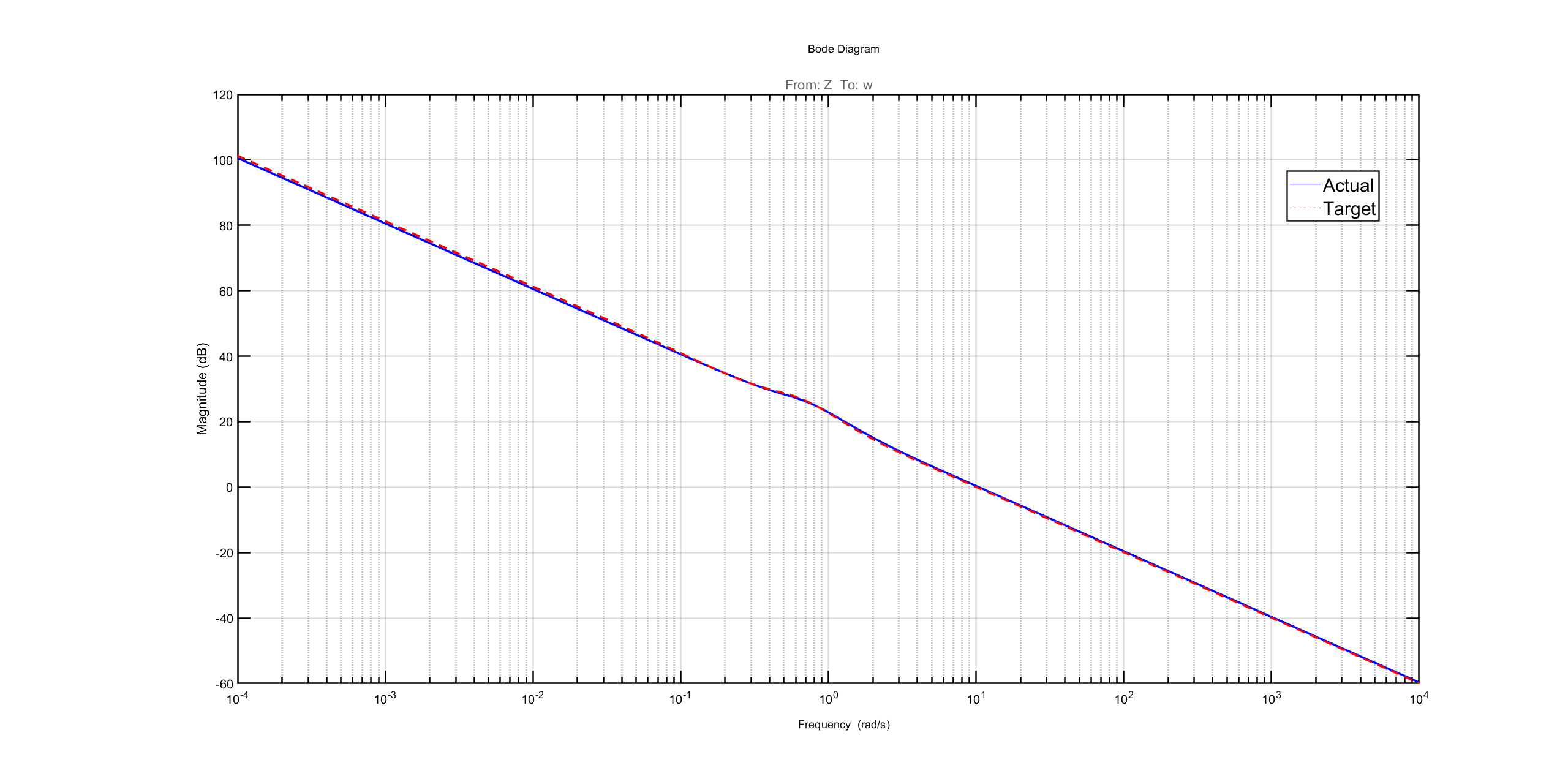
Plant
Continuous-time transfer function from depth \(z\) to heave speed \(w\):
\[G_{zw} = \frac{0.02082 s^3 + 0.1093 s^2 + 0.1083 s + 0.02464}{s^4 + 5.971 s^3 + 8.153 s^2 + 5.227 s + 1.541}\]
Controller
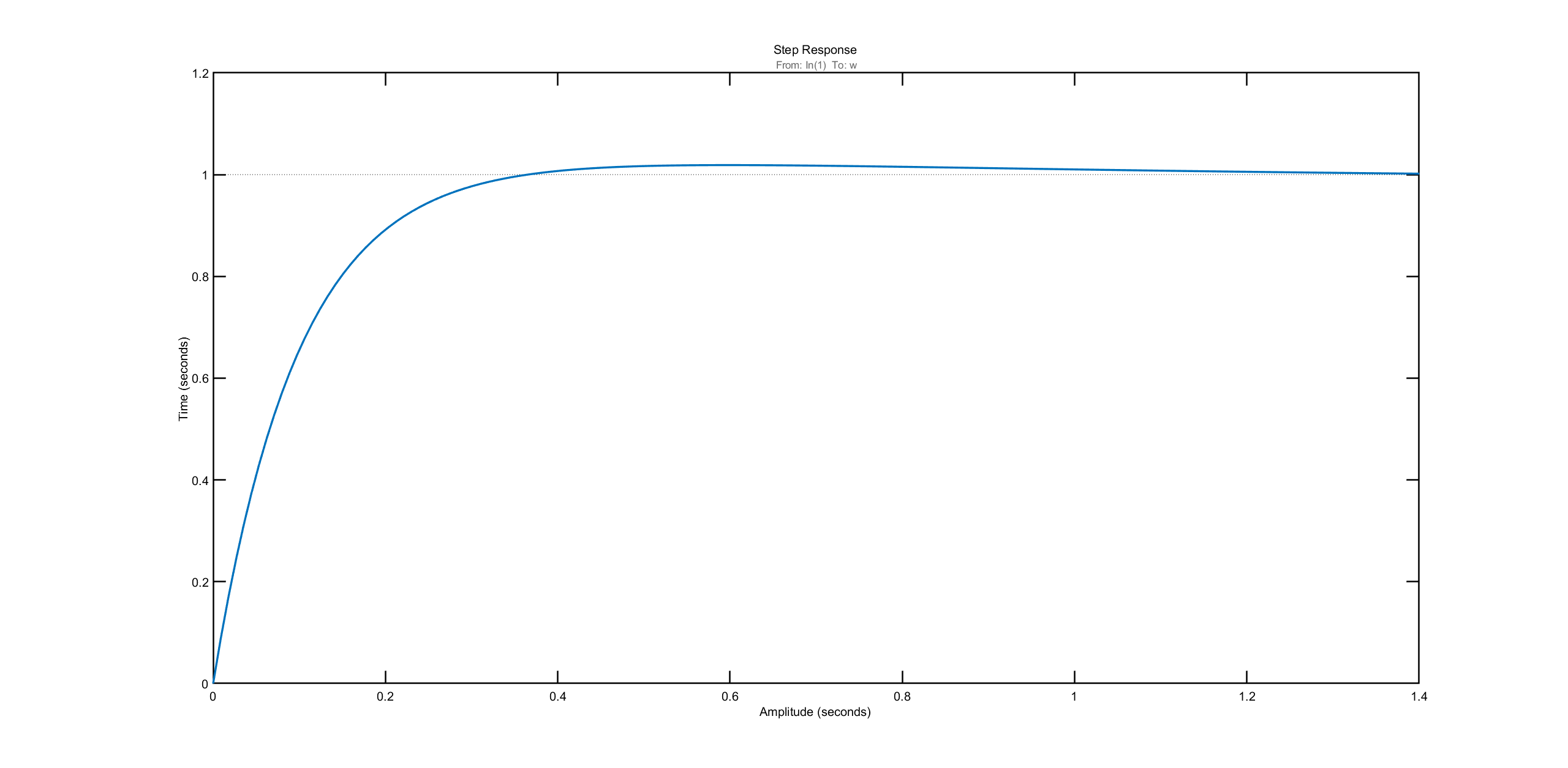
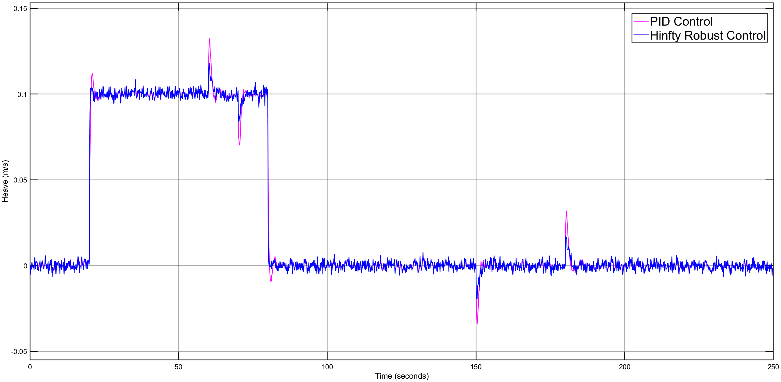
Performance
The \(H_{\infty}\) controller we designed shows better robustness and compatibility compared to PID:
Conclusion
The classical Loop Shaping robust control algorithm requires specific weighting functions for each controller. For instance, in mixed sensitivity design, weighting functions \(W_p(s)\), \(W_u(s)\), and \(W_T(s)\) are needed for \(S\), \(KS\), and \(T\) respectively, to complete the loop design. These functions must satisfy various constraints, such as \(\left\Vert S \right\Vert_\infty \le \gamma | W_P^{-1} |\), \(\left\Vert KS \right\Vert_\infty \le \gamma | W_u^{-1} |\), \(\left\Vert T \right\Vert_\infty \le \gamma | W_T^{-1} |\), \(T = GKS\), and \(S + T = 1\) etc., complicating their selection and making them crucial in the design process.
Glover and McFarlane proposed using the open-loop Bode plot for pre-weight and post-weight functions, simplifying design but requiring separate weights for MIMO systems. Safonov and Le introduced a method using all-pass squaring-down to compute the stable minimum-phase pre-weight function \(W(s)\), approximating the desired loop shape \(L(j\omega) \) without changing the system’s right-half-plane poles and zeros. Combined with the Balanced Stochastic Truncation (BST) algorithm, this simplifies design and yields low-order controllers.