Attitude Estimation Using the Nonlinear Explicit Complementary Filter (NECF)
Date:
Magnetometer Calibration
Ellipse function
\[F(x,y) = ax^2 + bxy + cy^2 +dx + ey +f = 0\]with an ellipse-specific constraint
\[b^2 - 4ac < 0 \implies 4ac - b^2 = 1\]The polynomial \(F (x, y)\) is called the algebraic distance of the point (x, y) to the given conic.
Ellipsoid function
Standard Form
non-rotated( magnetic field’s three axes align with the Cartesian coordinate of magnetometer) and center at origin
\[\frac{(x-x_c)^2}{x_m^2} + \frac{(y-y_c)^2}{y_m^2} + \frac{(z-z_c)^2}{z_m^2} = 1\]General Form
\[ax^2 + by^2 + cz^2 + 2dxy + 2exz + 2fyz + 2gx + 2hy + 2iz + j = 0\]with some extra constrains to maintain an ellipsoid
Calibration Method
Classical Two Step Method
first fit a ellipsoid
hard iron compensation caused by Permanent magnets and magnetized objects, permanent magnetic field, constant in all directions, whose effect is the addition of a constant bias on the magnetometer output(bias of the ellipsoid center)
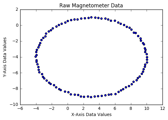
a. least squre fitting ellipse
\[\displaylines{ x_c = \frac{x_{max} + x_{min}}{2}\\ x_m = \frac{x_{max} - x_{min}}{2} }\]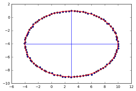
b. normalization
\[\large \begin{array}{c} x_{normalized} = \frac{x-x_c}{x_m}\\ y_{normalized} = \frac{y-y_c}{y_m} \end{array}\]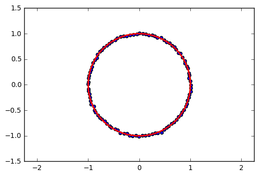
2. soft iron compensation(iduced magnetism) caused by ferromagnetic materials close to the sensor, whose magnitude is related to the angle of incidence of Earth’s magnetic field on the material itself, this effect changes as the orientation of the sensor varies. Stretching and tilting the sphere of ideal measurements. The resulting measurements lie on an ellipsoid 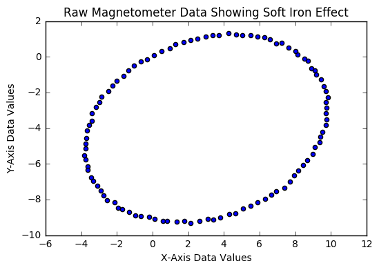
a. least squre fitting ellipse estimated values are same as hard iron 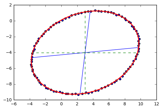
b. normalization
\[\large \begin{array}{c} x_{normalized} = x_m^{-1} \cdot (h_x-x_c)+a_{xy}^{-1} \cdot (h_y-y_c)+a_{xz}^{-1} \cdot (h_z-z_c)\\ y_{normalized} = a_{yx}^{-1} \cdot (h_x-x_c)+y_m^{-1} \cdot (h_y-y_c)+a_{yz}^{-1} \cdot (h_z-z_c)\\ z_{normalized} = a_{zx}^{-1} \cdot (h_x-x_c)+a_{zy}^{-1} \cdot (h_y-y_c)+z_m^{-1} \cdot (h_z-z_c) \end{array}\]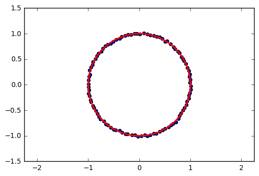
STMicroelectronics Calibration Method
\[\begin{array}{c} F(x, y, z) = ax^2 + by^2 + cz^2 + 2dxy + 2exz + 2fyz + 2gx + 2hy + 2iz = 1\\[2mm] v_{9\times1} = [a, b, c, d, e, f, g, h, i]^T\\[2mm] D_{n\times9} = [x^2, y^2, z^2, xy, xz, yz, x, y, z]\\[2mm] F_{n\times1} = Dv = \mathbf{1}_{n\times1} \end{array}\]least-square fitting(Linear Algebra pseudo-inverse)
\[\displaylines{ D^TDv = D_{9 \times n}^T\mathbf{1}_{n\times1}\\[1mm] v = (D^TD)_{9\times9}^{-1}(D\mathbf{1})_{9\times1} }\]- Origin Offset
2. De-rotate and Normalization
\[\displaylines{ T = \begin{bmatrix} 1 &0 &0 &0\\ 0 &1 &0 &0\\ 0 &0 &1 &0\\ o_x &o_y &0_z &1 \end{bmatrix}\\[1mm] B_{4\times4} = TAT^T = \begin{bmatrix}\begin{array}{ccc|c} b_{11} &b_{12} &b_{13} &b_{14}\\ b_{21} &b_{22} &b_{23} &b_{24}\\ b_{31} &b_{32} &b_{33} &b_{34}\\ \hline b_{41} &b_{42} &b_{43} &b_{44} \end{array}\end{bmatrix}\\[1mm] B_{3\times3} = -\frac{1}{b_{44}} \begin{bmatrix} b_{11} &b_{12} &b_{13}\\ b_{21} &b_{22} &b_{23}\\ b_{31} &b_{32} &b_{33} \end{bmatrix}\\[1mm] }\]\(A^T = A\) \(A\) is symmetric matrix,\(\exists\ A = Q \wedge Q^{-1} = Q \wedge Q^T \implies B_{4\times4} = TAT^T?\)
\[\displaylines{ \mathbf{Gain} = eigenvalues(B)\\[1mm] \mathbf{Rotation Matrix} = eigenvectors(B) }\]Freescale Semiconductor AN5019 Method
General Linear model
\[\displaylines{ ^S\mathbf{B}_k = \mathbf{W} ^S\mathbf{B}_{c,k} + \mathbf{V}\\[1mm] {}^S\mathbf{B}_{c,k} = \mathbf{W}^{-1} (^S\mathbf{B}_k - \mathbf{V})\\[1mm] {}^S\mathbf{B}_{c,k} = R{}^G\mathbf{B}_0\\[1mm] {}^S\mathbf{B}_k = \mathbf{W} R{}^G\mathbf{B}_0 + \mathbf{V} }\]Measurement Loci
Locus of calibrated magnetic field \({}^S\mathbf{B}_{c,k}\) is a sphere centered at origin with radius \(B\)
\[\left \Vert {}^S\mathbf{B}_{c,k} \right \Vert^2 = ({}^S\mathbf{B}_{c,k})^T {}^S\mathbf{B}_{c,k} = (R{}^G\mathbf{B}_0)^T R{}^G\mathbf{B}_0 = \left\Vert {}^G\mathbf{B}_0\right\Vert^2 = B^2\]Locus of uncalibrated magnetic field \({}^S\mathbf{B}_k\) is a ellipsoid:
\[\|{}^S\mathbf{B}_{c,k} \|^2 = \{ \mathbf{W}^{-1} (^S\mathbf{B}_k - \mathbf{V})\}^T \{\mathbf{W}^{-1} (^S\mathbf{B}_k - \mathbf{V})\} = (R{}^G\mathbf{B}_0)^T R{}^G\mathbf{B}_0 = B^2\\[1mm] (^S\mathbf{B}_k - \mathbf{V})^T(W^{-1})^TW^{-1} (^S\mathbf{B}_k - \mathbf{V}) = B^2\]general expression of a ellipsoid:
\[(u-u_o)^T A (u-u_0)=const\\[1mm] (^S\mathbf{B}_k - \mathbf{V})^T A (^S\mathbf{B}_k - \mathbf{V}) = B^2\]\(u\) is the sampled track points \(u_0\) is the center of ellipsoid let \(A =(W^{-1})^TW^{-1}\) , then \(A\) is a symmetric matrix denoting the shape characteristics of ellipsoid
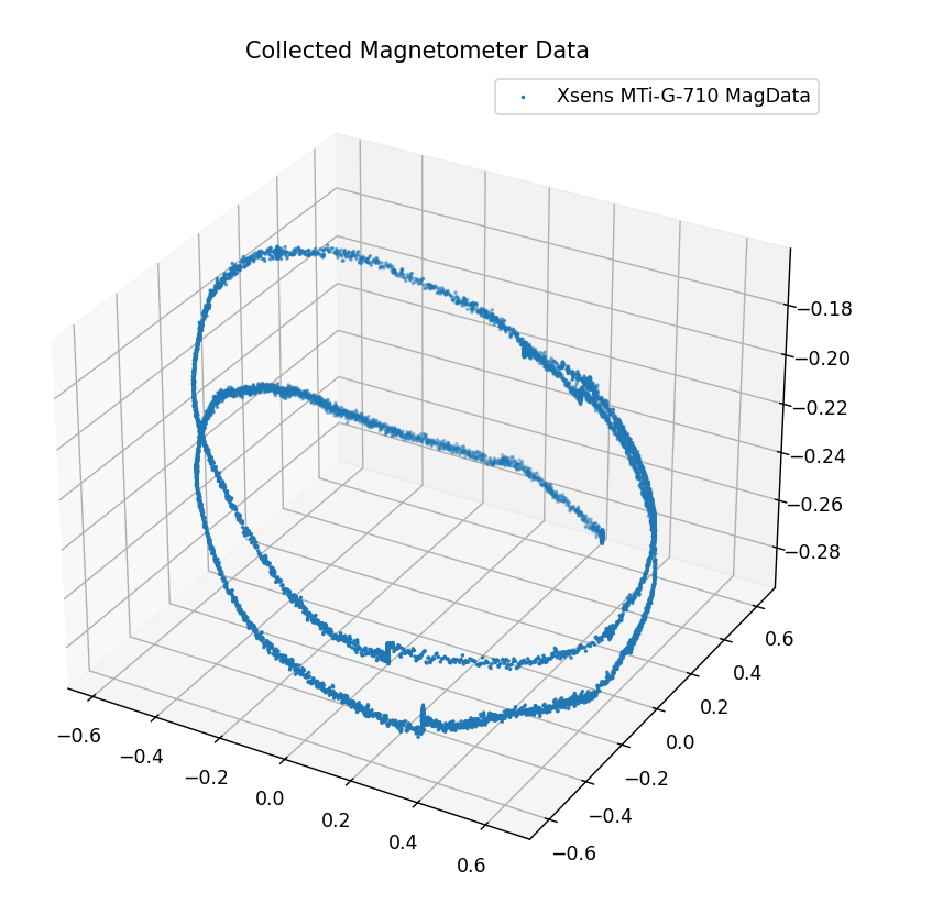
Now we can say, if we can fit the locus of sampled magnetometer readings to a ellipsoid, we can find out the offset of hard iron effect by calculate the average magnetic magnitude of each axe, which is \(u_o\), and we can then use the known conditions to estimate soft iron interference rotation matrix \(W\).
Least Square Error Optimization
\[\displaylines{ r_k = \|{}^S\mathbf{B}_{c,k}\|^2 - B^2 = (^S\mathbf{B}_k - \mathbf{V})^TA (^S\mathbf{B}_k - \mathbf{V}) - B^2 \implies r_k = Y_k - X_k\beta = 0\\[1mm] i.e.\ \mathbf{r} = \mathbf{Y} - \mathbf{X}\mathbf{\beta} \implies X\beta = Y }\]use least square to find the solution \(\beta\), find the least sum of square error \(E(\beta)\):
\[\begin{align*} E(\beta) = \|\mathbf{r}\|^2 &= (Y-X\beta)^T(Y-X\beta) =Y^TY -Y^TX\beta - \beta^T X^TY + \beta^TX^TX\beta\\ &=Y^TY + \beta^TX^TX\beta - 2\beta^T X^TY \end{align*}\] \[\lim_{\delta \beta \to 0} \frac{E(\beta + \delta\beta) -E(\beta) }{\delta\beta} = 0 \implies \beta = (X^TX)^{-1}X^TY\]Homogeneous(both hard and soft compensation)
\(Y_k = 0\), original function will only get useless zero solution, we use lagrange multiply instead, by giving a constrain \(g(x) = c\):
\[\displaylines{ \beta^T\beta = 1\\[1mm] L = E(\beta) + \lambda(\beta^T\beta-1) \implies X^TX\beta = \lambda \beta }\]the required solution vector is one of the eigenvectors of the product matrix \(X^TX\) with eigenvalue \(\lambda\).
\[E(\beta) = \beta^TX^TX\beta = \lambda \beta^T\beta = \lambda\]The minimum error function is therefore equal to the smallest eigenvalue \(\lambda_{min}\) of \(X^TX\) and the required solution \(\beta_{min}\) is the eigenvector with the smallest eigenvalue.
- non-rotated ellipsoid(soft iron effect only shows on stretching)
omit
2. rotated ellipsoid(both stretching and tilting)
\[\displaylines{ A = \begin{bmatrix} A_{xx} &A_{xy} &A_{xz}\\ A_{xy} &A_{yy} &A_{yz}\\ A_{xz} &A_{yz} &A_{zz} \end{bmatrix} }\] \[\displaylines{ \beta_{min} = [\beta_0, \beta_1, \beta_2, \beta_3, \beta_4, \beta_5, \beta_7, \beta_8, \beta_{9}]^T\\[1mm] A = \begin{bmatrix} \beta_0 &\beta_1 &\beta_2\\ \beta_1 &\beta_3 &\beta_4\\ \beta_2 &\beta_4 &\beta_5 \end{bmatrix}\\[1mm] V = -\frac{1}{2}A^{-1}\begin{pmatrix}\beta_6\\ \beta_7\\ \beta_8\end{pmatrix}\\[1mm] W^{-1} = \sqrt{A} }\]Non-Homogeneous(only hard iron compensation)
\(Y_k \ne 0\), overlook here
\[\beta = (X^TX)^{-1}X^TY\]2D Planar Calibration
- Minimal Distance Plane and Magnetic Projection
if all points lie on the plane, then \(e = 0 \in R^n×1\), so this actually is another homogeneous least square error question, we just need to find the optimal solution corresponds to: \(|e|^2 = |e^Te| = |A^TQ^TQA|\) The only different this time is using singular value decomposition(SVD) to solve this least square question. The solution of such system is the closest vector to the kernel of \(Q\), which is given by the right-singular vector corresponding to the minimum singular value obtained from the SVD of \(Q\). And the reason shows in SVD求解线性方程组.
\[m^p = m + tn = m - \frac{n^T(m - P)}{\|n\|}n\]If normal \(n\) is an unit vector, then \(m_p = m - {\underbrace{n^T(m - P)}_{const}}n\)
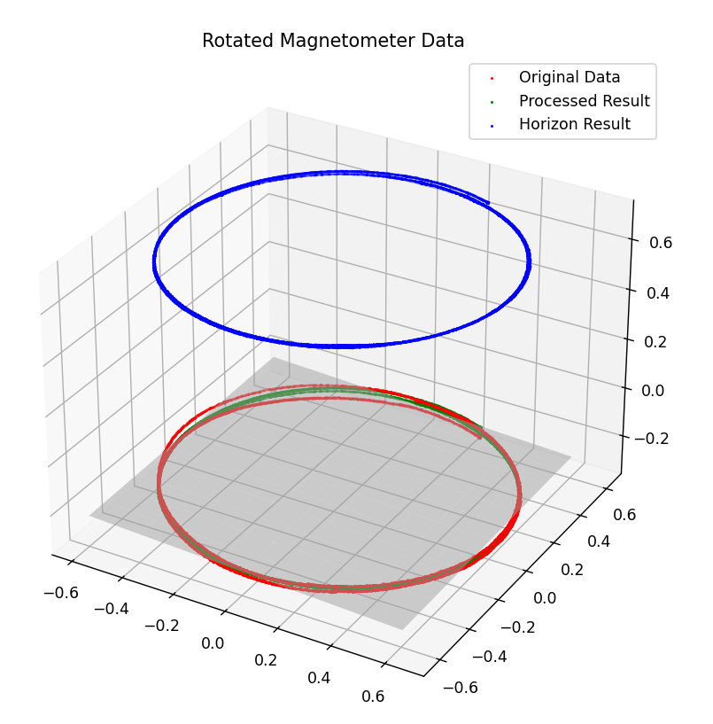
2. Horizontal Alignment
\[\displaylines{ m^h = R(\theta, \alpha)m^p\\[2mm] \alpha = n \times z = \begin{vmatrix} i &j &k\\ n_x &n_y &n_z\\ 0 &0 &1 \end{vmatrix} = n_y i - n_x j = [n_y, n_x, 0]^T\\[1mm] \theta = arccos(n\cdot z) = arccos(z^Tn) }\]It seems that if we let \(\theta \in [0, \frac{\pi}{2}]\) then \(\theta\) will be negtive when it exceeds \(\frac{\pi}{2}\), and we rotate adversely about the spin-axi for negtive angle, then we don’t need to calculate the normal vector \(n^{out}\) that points to the half-space. Axis–angle representation
3. Radim HalII 2D Ellipse Fitting Though this method we can get the characteristics of a general ellipse and we can use geometric knowledge to calculate the corresponding semi-axial length and the rotation angle by 一般椭圆方程标准化及其推导 or wiki ellipse
Reference
- 三维空间中的椭球拟合+磁力计校准算法+加速度计校准算法
- How to Calibrate a Magnetometer
- agnetic calibration methods defination
- A way to calibrate a magnetometer
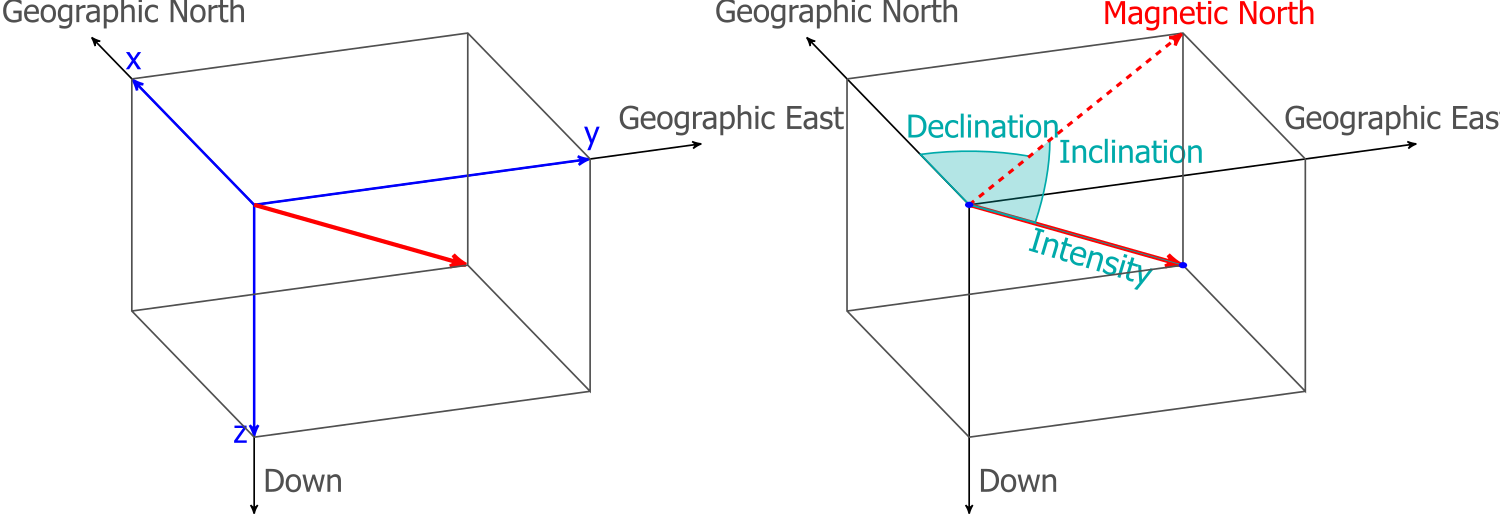
Latitude, Longitude, Elevation, and Magnetic Field
C栋:22.588642995403102N, 113.96927123871706E 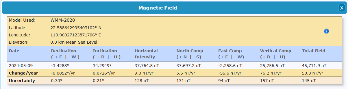
Least Square Optimization
Least Squares Solution of Overdetermined Systems
\[\displaylines{ Ax = b\\ A^TAx = A^Tb\\ x = (A^TA)^{-1} A^Tb }\]\(b\): observations(dependent)
\(A\): input coefficient matrix(independent)
\(x\): unknown variables
The concept of the least squares solution for a system of linear equations, as discussed in this article, relies on Singular Value Decomposition (SVD). This solution, also known as the Normal Equations solution, minimizes the sum of the squares of the errors. The objective function, being a positively parameterized multivariate quadratic equation, has a unique minimum. The target solution is found by deriving and solving this objective function.
NECF Mehod
Madgwick’s implementation of Mayhony’s AHRS algorithm
Magnetic distortion compensation
Madgwick let the desired magnetic field direction turn from \(m^n = [h_x, h_y, h_z]^T\) to \([\sqrt{h_x+h_y}, 0, h_z]^T\), so the cross product of \(m_c^b\) would eliminate the influence of magnetic inclination.
\[\begin{align*} error &= m_c^b \times \hat{m}_c^b \\ &= \{ (m_c^b)_{||} + (m_c^b)_{\perp} \} \times \{ (\hat{m}_c^b)_{||} + (\hat{m}_c^b)_{\perp} \}\\ &= (m_c^b)_{||} \times (\hat{m}_c^b)_{||} + (m_c^b)_{||} \times (\hat{m}_c^b)_{\perp} + (m_c^b)_{\perp} \times (\hat{m}_c^b)_{||} + (m_c^b)_{\perp} \times (\hat{m}_c^b)_{\perp} \\ &= (m_c^b)_{||} \times (\hat{m}_c^b)_{||} + (m_c^b)_{\perp} \times (\hat{m}_c^b)_{\perp}\\ &= \underbrace{ \delta declination}_{Non-compensable} + \underbrace{\delta inclination}_{compensable} \implies \delta heading + 0\\ \end{align*}\]Madgwick try to let the \(\delta_{incl}\) be zero, by letting \(\hat{m}_c^b = [\sqrt{h_x+h_y}, 0, h_z]^T\) to ensure there is no error in inclination angle and the error between the desired magnetic direction and the sensor measured direciton is exactly the declination angle, by which the NECF can mainly deal with the heading error.
Costanzi’s NECF implementation
Find details in An Attitude Estimation Algorithm for Mobile Robots Under Unknown Magnetic Disturbances. This paper optimizes underwater robot attitude estimation by compensating for quantifiable magnetic disturbance and using FOG to enhance accuracy during unpredictable interference. Sensor rotation disturbance is fully compensable, while external environmental interference is not. We also utilize Random Sample Consensus (RANSAC) to eliminate outliers, and the results are as follows: